# 代码来源:https://www.r2omics.cn/
library(circlize)
library(ComplexHeatmap)
library(magrittr)

cheatmap = function(
    df = NULL,               # 主数据框(矩阵形式,行为特征,列为样本)
    dfSample = NULL,         # (可选)样本分组信息(两列数据框:Sample列和Group列)
    group_colors = NULL,     # 自定义分组颜色向量(命名向量)
    scale = "row",           # 数据标准化方式:none(不处理)/row(行标准化)/column(列标准化)
    col_fun = NULL,          # 自定义颜色映射函数(由colorRamp2创建)
    # 聚类控制参数
    cluster_rows = TRUE,     # 是否对行聚类
    cluster_cols = TRUE,     # 是否对列聚类
    clustering.method  = "complete",  # 聚类方法(hclust方法)
    distance.method  = "euclidean",   # 距离计算方法
    # 可视化参数
    dend.track.height  = 0.1, # 树状图轨道高度
    show_rownames = TRUE,    # 显示行名
    show_colnames = TRUE,    # 显示列名
    legend_font_size = 10,
    legend_value_name = "",
    legend_group_name = "Group",
    font_size = 0.5,         # 标签字体大小
    track.height  = 0.3,      # 热图轨道高度
    start.degree  = 0,        # 环形起始角度
    gap.degree  = 30          # 扇区间隔角度
){
  # 归一化
  if(scale=="row"){
    # 按行归一化
    dfNormalize = t(scale(t(df))) %>% as.data.frame()
  }else if(scale=="column"){
    # (或)按列归一化
    dfNormalize = scale(df) %>% as.data.frame()
  }else if(scale=="none"){
    dfNormalize = df
  }else{
    stop("scale参数不正确,选择none row column中的一种")
  }

  # 设置颜色
  if(is.null(col_fun)){
    col_fun = colorRamp2(c(floor(min(dfNormalize,na.rm=T) ),
                           0,
                           ceiling(max(dfNormalize,na.rm=T))),
                         c("#0000ff", "#ffffff", "#ff0000"))
  }

  circos.par(start.degree  = start.degree, gap.degree  = gap.degree)


  if(cluster_cols){
    column_od <- hclust(dist(t(dfNormalize),method = distance.method),method = clustering.method)$order
    dfPlot = dfNormalize[,  column_od]
  }else{
    dfPlot = dfNormalize
  }

  if(cluster_rows){
    dend.side = "inside"
  }else{
    dend.side = "none"
  }

  if(show_rownames){
    rownames.side = "outside"
    my.track.index = 2
  }else{
    rownames.side = "none"
    my.track.index = 1
  }

  circos.heatmap(dfPlot,
                 track.height  = track.height,
                 cluster = cluster_rows,
                 clustering.method  = clustering.method,
                 distance.method  = distance.method,
                 rownames.side  = rownames.side, # c("none", "outside", "inside"),
                 rownames.cex  = font_size,
                 rownames.font  = par("font"),
                 rownames.col  = "black",
                 dend.callback  = function(dend, m, si) reorder(dend, rowMeans(m)),
                 # dend.callback  = function(dend, m, si) {{dendsort::dendsort(dend)}},
                 dend.side  = dend.side,
                 dend.track.height  = dend.track.height,
                 col = col_fun
  )


  if(is.null(dfSample)){

  }else{
    # 获取样本分组信息
    colnames(dfSample) = c("Sample", "Group")

    sample_groups <- dfSample$Group[match(colnames(dfPlot), dfSample$Sample)]
    unique_groups <- unique(sample_groups)

    if(is.null(group_colors)){
      group_colors <- setNames(c("#bfff7f", "#8ec7ff", "#ffc57f", "#f18c8d","#ea4436","#000000"), unique_groups)
    }

    # 为每个样本添加条带
    circos.track(
      track.index  = my.track.index,
      panel.fun  = function(x, y) {
        if(CELL_META$sector.numeric.index  == 1) {
          cn = colnames(dfNormalize[, column_od])
          n = length(cn)
          for(i in 1:n) {
            group <- sample_groups[i]
            color <- group_colors[group]
            circos.rect(
              0 - convert_x(1, "mm"), i - 1,
              0 - convert_x(5, "mm"), i,
              col = color, border = NA
            )
          }
        }
      },
      bg.border  = NA
    )
  }


  if(show_colnames){
    circos.track(
      track.index =my.track.index,
      panel.fun = function(x, y) {
        if (CELL_META$sector.numeric.index == 1) {
          # 在最后一个扇形中
          cn = colnames(dfNormalize[, column_od])
          n = length(cn)
          circos.text(
            rep(CELL_META$cell.xlim[2], n)  + convert_x(1, "mm"),
            1:n -0.5,
            cn,
            cex = font_size,
            adj = c(0, 0.5),
            facing = "inside"
          )
        }
      },
      bg.border = NA
    )
  }


  circos.clear()

  lgd_heatmap <- Legend(title = legend_value_name, col_fun = col_fun,
                        labels_gp = gpar(fontsize = legend_font_size),
                        title_gp = gpar(fontsize = legend_font_size, fontface = "bold")#,
                        # grid_height = unit(10, "mm"),
                        # grid_width = unit(2, "mm"),
                        # legend_height  = unit(10, "mm"),
                        # legend_width  = unit(3, "mm")
                        )
  # 创建图例对象
  if(is.null(dfSample)){
    pd <- packLegend( lgd_heatmap,
                      direction = "horizontal", gap = unit(0, "cm"))
  }else{

    lgd_groups <- Legend(labels = names(group_colors), title = legend_group_name,
                         legend_gp = gpar(fill = group_colors),
                         labels_gp = gpar(fontsize = legend_font_size),
                         title_gp = gpar(fontsize = legend_font_size, fontface = "bold")#,
                         # grid_height = unit(10, "mm"),
                         # grid_width = unit(2, "mm"),
                         # legend_height  = unit(10, "mm"),
                         # legend_width  = unit(3, "mm")
                         )
    # 组合图例并设置间距
    pd <- packLegend( lgd_heatmap, lgd_groups,
                      direction = "horizontal", gap = unit(1, "cm"))
  }
  # 统一绘制
  draw(pd, x = unit(0.5, "npc"), y = unit(0.5, "npc"))

}R语言如何绘制圆形热图
前言
本篇是R语言circlize包和ComplexHeatmap包绘制圆形热图的教程。circlize包语法较为生涩,故整理个自定义函数,方便调用。
什么是圆形热图?
热图是是一种将规则化矩阵数据转换成颜色色调的常用的可视化方法,其中每个单元格对应数据的某些属性,属性的值通过颜色映射转换为不同色调并按规则填充单元格。
圆形热图简单说就是,将传统矩形热力图转化为环形布局的数据可视化形式。
绘图前的数据准备
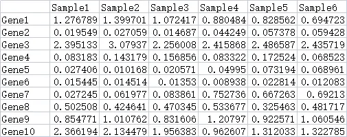
热图数据
数据来源一般是搜库结果定量表。包含2个维度的数据,一般情况下,每一行是一个基因,每一列是一个样本。
demo数据可以在https://www.r2omics.cn/res/demodata/heatmap/data.heatmap.txt下载。
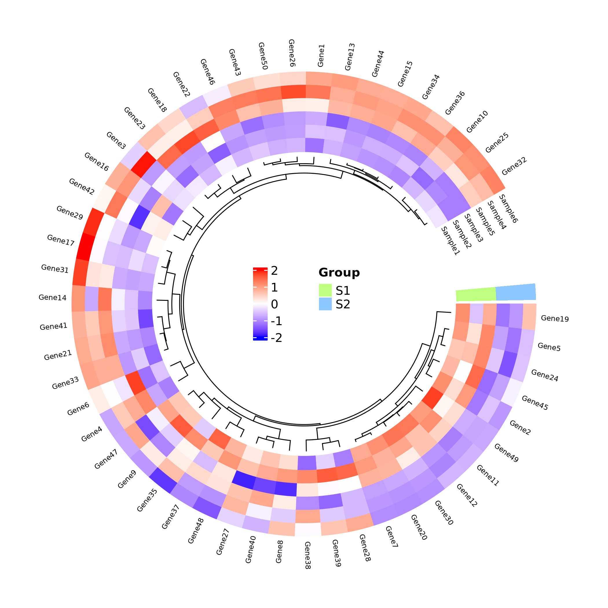
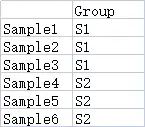
样本分组数据(可选)
行名的名称和个数要和之前的heatmap数据保持一致,列名为分组名称,可以包含不止一个分组。
demo数据可以在https://www.r2omics.cn/res/demodata/heatmap/sample.class.txt下载。
R语言如何绘制圆形热图
加载配置自定义函数,之后直接调用即可
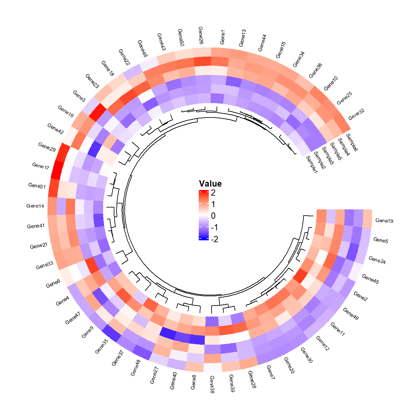
调用函数绘图
# 代码来源:https://www.r2omics.cn/
# 读取数据
df = read.delim("https://www.r2omics.cn/res/demodata/heatmap/data.heatmap.txt",  row.names  = 1)
# 样本分组(可选)
# dfSample = read.delim("https://www.bioladder.cn/shiny/zyp/demoData/heatmap/sample.class.txt")

# 绘图
cheatmap(
  df = df,                  # 主数据框(矩阵形式,行为特征,列为样本)
  # dfSample = dfSample,    # (可选)样本分组信息(两列数据框:Sample列和Group列)
  group_colors = NULL,      # 自定义分组颜色向量
  scale = "row",            # 数据标准化方式:none(不处理)/row(行标准化)/column(列标准化)
  col_fun = NULL,           # 自定义颜色映射函数(由colorRamp2创建)
  cluster_rows = T,         # 是否对行聚类
  cluster_cols = TRUE,      # 是否对列聚类
  clustering.method  = "complete", # 聚类方法(hclust方法)
  distance.method  = "euclidean",  # 距离计算方法
  dend.track.height = 0.1,  # 树状图轨道高度
  show_rownames = T,        # 显示行名
  show_colnames = TRUE,     # 显示列名
  font_size = 0.5,          # 标签字体大小
  legend_font_size = 10,    # 图例字体大小
  legend_value_name = "Value", # 图例标题
  legend_group_name = "Group", # 分组图例标题
  track.height = 0.3,       # 热图轨道高度
  start.degree  = 0,        # 环形起始角度
  gap.degree  = 30          # 扇区间隔角度
)